Simulation Study

I’m hiding the simulator functions, as the code is kludgy, similar to the 2020-01-19 post, and not the point, but you can find the source .Rmd on github.

To make things interesting, the simulation simply extends the interference simulation by adding additional timepoints for each subject. The outcomes can depend on the unit’s exposure (and that of neighbors) from the current and previous timepoint, as well as the outcome from the previous timepoint. To get time-varying confounding, a unit’s exposure also depends on the previous exposure.

Generic Permutation Weighting Functions

#' Stack the observed data with the permuted data
#' @export
permute_and_stack <- function(dt, permuter){
  dplyr::bind_rows(
    dplyr::mutate(dt,  C = 0),
    dplyr::mutate(permuter(dt), C = 1)
  ) 
}

#' Estimate the density ratio by modeling whether an observation is from 
#' the permuted dataset or original dataset
.pw <- function(dt, rhs_formula, fitter, modify_C, predictor, fitter_args, permuter){
  pdt <- permute_and_stack(dt, permuter)
  pdt$C <- modify_C(pdt$C)
  m  <- do.call(
    fitter,
    args = c(list(formula = update(C ~ 1, rhs_formula), data = pdt), fitter_args))
  
  w  <- predictor(object = m, newdata = dt) 
  w/(1 - w)
}

#' Estimate permutation weights B times and average the results
#' @export
get_permutation_weights <- function(dt, B, rhs_formula, fitter, modify_C = identity, 
                                    predictor, fitter_args = list(),
                                    permuter){
  out <- replicate(
    n    = B,
    expr = .pw(dt, rhs_formula = rhs_formula, fitter = fitter, modify_C = modify_C,
               predictor = predictor, fitter_args = fitter_args,
               permuter = permuter)
  )
  
  apply(out, 1, mean)
}

#' Create a permutation weighted estimator for the marginal structural model
#' @export
make_pw_estimator <- function(fitter, rhs_formula, B, 
                              modify_C = identity,
                              predictor = function(object, newdata) {
                                predict(object = object, newdata = newdata, type = "response") 
                              },
                              fitter_args = list(),
                              permuter){
  function(data){
    
    w <- get_permutation_weights(
      dt = data, B = B, rhs_formula = rhs_formula, fitter  = fitter,
      modify_C = modify_C, predictor = predictor, fitter_args = fitter_args,
      permuter = permuter
    )
    
    w
  }
}

Specific PW functions

These functions are specific for analyzing the data simulated for this post. Note that the permuting function permutes entire vectors of treatment. Also the binary classifier used in the permutation weighting estimator uses a GEE model.

# Half ass permutation attempt with several poor practices
# * number of timepoints is hardcoded!
# * number of timepoints is same for all subjects
# * object `edges` will need to be found in an another environment (i.e. Global)
permuterf <- function(dt){
  dt <- dplyr::arrange(dt, id, t)
  rl <- rle(dt$id)
  permutation <- rep((sample(rl$values, replace = FALSE) - 1L) * 4L, each = 4L) + 1:4
  dt %>%
    dplyr::mutate(
      A = A[permutation]
    ) %>%
    dplyr::group_by(t) %>%
    dplyr::mutate(
      # Number of treated neighbors
      A_n = as.numeric(edges %*% A),
      # Proportion of neighbors treated
      fA  = A_n/m_i,
      id  = id + max(id)
    ) %>%
    dplyr::ungroup() %>%
    dplyr::group_by(id) %>%
    dplyr::mutate(
      Al  = dplyr::lag(A),
      fAl = dplyr::lag(fA)
    ) %>%
    dplyr::ungroup() 
}

gee_fitter <- function(formula, data, ...){
  data <- dplyr::filter(data, t > 0)
  geepack::geeglm(formula = formula, data = data, id = id, family = binomial)
}

pdct <- function(object, newdata) { 
  predict(object = object, newdata = dplyr::filter(newdata, t > 0), type = "response")
}

Here’s the estimator I’ll use:

pw_geeimator <- make_pw_estimator(
  gee_fitter,
  B = 5,
  rhs_formula = ~ ((A + fA + Al + fAl):(factor(t) + Z1_abs*Z2 + Z3 + Yl) +
                  (factor(t) + Z1_abs*Z2 + Z3 + Yl)),
  permuter = permuterf,
  predictor = pdct)

# Fix an adjacency matrix for use across simulations
# Set sample size to 5000
edges <- gen_edges(n = 5000, 5)

sim_data <- function(){
   edges  %>%
   gen_data_0(
        gamma = c(-2, 0.2, 0, 0.2, 0.2),
        beta = c(2, 0, 0, -1.5, 2, -3, -3)
    ) %>%
    purrr::reduce(
      .x = 1:3, # 3 timepoints after time 0
      .f = ~ gen_data_t(.x, .y,           
                        gamma = c(-2, 3, 0, 0.2, 0, 0.2, 0.2),
                        beta  = c(2, 0, 0, 0, -0.5, 0, -1.5, 2, -3, -3)),
      .init = .
    ) %>%
    purrr::pluck("data") %>%
    dplyr::arrange(id, t)
}

do_sim <- function(){
  dt <- sim_data()
  w  <- pw_geeimator(dt)
  dt <- dt %>% dplyr::filter(t > 0) %>% dplyr::mutate(w = w)
  
  res_w <- geepack::geeglm(
    Y ~ -1 + factor(t) + A + Al + fA + fAl, data = dt, id = id, weights = dt$w
  )
  
  res_naive <- geepack::geeglm(
    Y ~ -1 + factor(t) + A + Al + fA + fAl, data = dt, id = id
  )
  
  
  bind_rows(
    broom::tidy(res_naive) %>% dplyr::mutate(estimator = "naive"),
    broom::tidy(res_w) %>% dplyr::mutate(estimator = "pw_weighted")
  )
  
}

In the sim_data function, I set the parameters so that the only non-null effect is the exposure of neighbors from the previous timepoint.

Results

The plot below shows the bias from 100 simulations for the 4 causal parameters from a naive (unweighted) GEE model and the permutation weighted version.

library(dplyr)
## 
## Attaching package: 'dplyr'
## The following objects are masked from 'package:stats':
## 
##     filter, lag
## The following objects are masked from 'package:base':
## 
##     intersect, setdiff, setequal, union
library(geepack)
library(ggplot2)

res <-
  purrr::map_dfr(1:100, ~ do_sim(), .id = "simid") %>%
  filter(grepl("A", term)) %>%
  group_by(simid) %>%
  mutate(
    bias = estimate - c(0, 0, 0, -0.5)
  )
  
ggplot(
  data = res,
  aes(x = estimator, y = bias)
) +
  geom_hline(yintercept = 0) +
  geom_jitter() +
  facet_grid(~ term)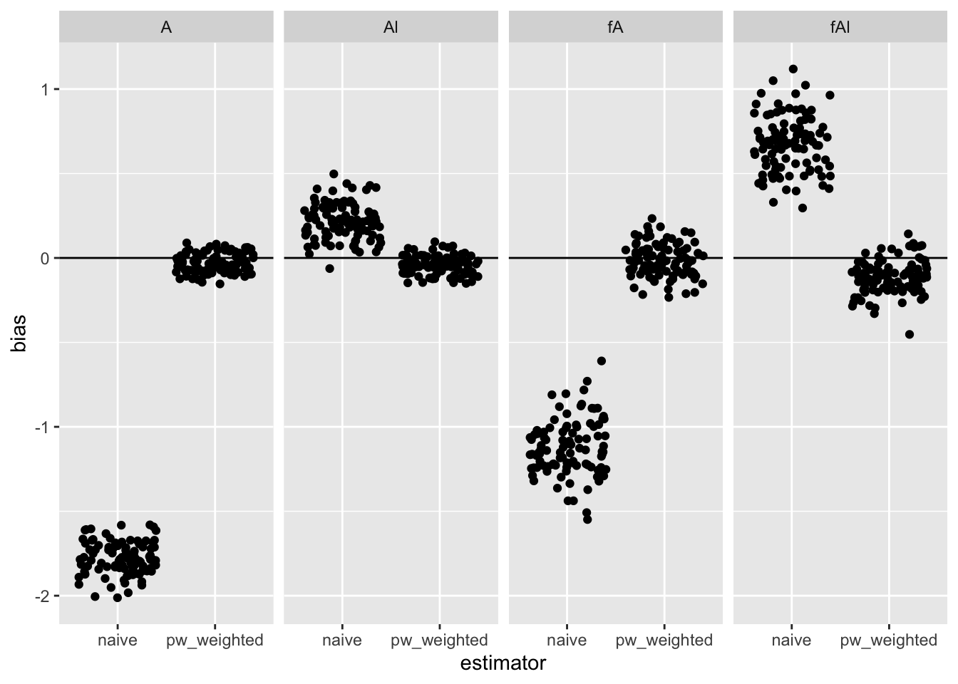

Summary

• Even after adding a time element to interference simulation from the other day, permutation weighting still works. I’m not surprised.
• The estimate for the non-null fAl appears downwardly biased a bit. I’ll want to look into that further, but in general permutation weighting seems like a promising approach.