Simulator functions

I’ve written two key functions: create_model_simulator and create_simulator. The create_model_simulator function fits a gam model and returns a function (technically a closure) which can take new data as well as update parameters. Out of laziness, I’m updating parameters based on names, but if I were shipping this function I would clean it up quite a bit.

The post argument takes a function that can be used to modify the final output. I use this pattern a lot in my R programming: including an option to post (and/or pre) processing output (and/or input) from/to a function.

create_model_simulator <- function(formula, data, family, post = identity){
  m    <- mgcv::gam(formula = formula, data = data, family = family)
  fm   <- formula(m)
  beta <- coef(m)
  inv  <- family()[["linkinv"]]
  function(newdata, newparms){
    X <- mgcv::gam(fm, data = newdata, family = family(), fit = FALSE)[["X"]]
    beta[names(newparms)] <- newparms
    post(inv(X %*% beta))
  }
}

Now I create simulator for the exposure and the outcome. The models are somewhat complicated in terms of the functional form of the predictors, but I don’t want a model too complicated with hundreds of parameters, as I prefer predictions to be computationally fast.

# Prediction models for simulation
exposure_simulator <- 
  create_model_simulator(
    formula = A ~ log(ha)*slope + 
      I(p_wet == 0) + p_wet + 
      I(neighbor_p_wet == 0) + neighbor_p_wet + 
      log1p(coast_2500) + travel +
      s(log(ha)) +
      s(slope) + 
      s(p_wet) + 
      s(travel),
    data   = basisdt,
    family = binomial,
    # Generate 0/1 exposure
    post   = function(x) { rbinom(length(x), size = 1, prob = x) }
  )

outcome_simulator <- create_model_simulator(
  formula = d_forested ~
    A*A_tilde + 
    log(ha)*slope +
    I(p_wet == 0) + p_wet +
    I(neighbor_p_wet == 0) + neighbor_p_wet + 
    log1p(coast_2500) + travel +
    s(log(ha)) +
    s(slope) +
    s(p_wet) +
    s(travel),
  data   = basisdt,
  family = gaussian,
  # inv(X %*% beta) returns a 1D matrix, but I need a vector so drop
  post   = drop
)

The create_simulator function take the two model simulators above to produce function that can a simulated dataset given covariate data and optionally new parameters. In my case, the function is more complicated than simply simulating the exposure and outcome. The \(f(\tilde{A})\) term needs to be recomputed after the exposure is generated but before the outcome is generated. Here, \(f(\tilde{A})\) is the proportion of a parcel’s boundary shared with treated parcels, thus in addition to covariates the basis data for a simulation needs to contain covariates plus parcel adjacency information (neighbor_pids in the code below).

create_simulator <- function(exposure_sim, outcome_sim){
  force(exposure_sim)
  force(outcome_sim)
  function(newdata, exposure_newparms = NULL, outcome_newparms = NULL){
    df <- newdata
    df[["A"]] <- exposure_sim(df, exposure_newparms)
    df %>%
      {
        hold  <- .
        
        dplyr::mutate(
          hold,
          # Update treatment of neighbors
          tr_neighbors = purrr::map(
            .x = neighbor_pids,
            .f = ~ hold[["A"]][hold[["pid"]] %in% .x]
          )
        )
      } %>%
      dplyr::mutate(
        # Proportion of boundary shared with treated units
        A_tilde = purrr::map2_dbl(
          .x = tr_neighbors,
          .y = neighbor_boundary_lengths,
          .f = function(x, y){
            `if`(length(x) == 0 || sum(as.numeric(y)) == 0, 
                 0, sum(x * y)/sum(y))
          })
      ) ->
      df
    df[["Y"]] <- outcome_sim(df, outcome_newparms)
    
    df
  }
}

Now I can create my simulator:

simulator1 <- create_simulator(exposure_simulator, outcome_simulator)

An advantage of having create_simulator return a closure is that I can save this closure to disk for use later within needing to refit models and reload large datasets.

Sampling

I sample 3000 parcels. I may not need all these in the end, but better to sample extra now than need to go back later.

frame <- sf::as_Spatial(sf::st_cast(basisdt$geometry, "POLYGON"))
smpl  <- SDraw::sdraw(frame, n = 3000, type = "BAS")
ids   <- basisdt$pid[as.integer(gsub("ID", "", smpl$geometryID))]

The sample indeed looks like Massachusetts:

plot(basisdt$geometry[basisdt$pid %in% ids])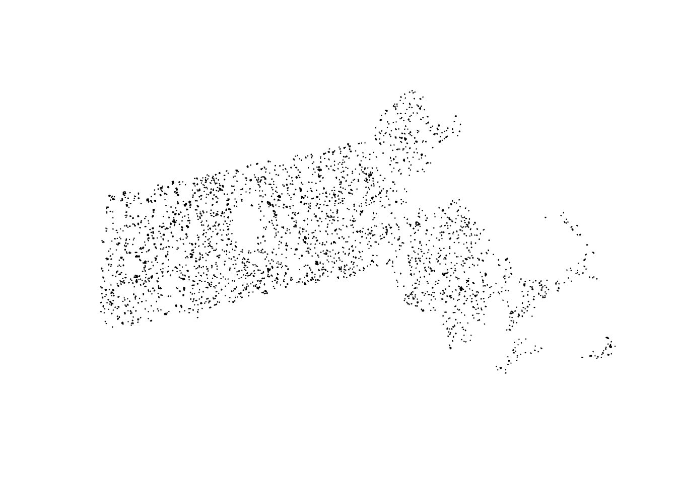

Usage

Now that I have “seed” parcels, I create simulated datasets by drawing a circle around a sampled parcel and taking all the parcels that are within or intersect the buffer. Creating the basis for a simulation requires an extra step here because the neighbors need to be updated after the sample is taken since all of a parcel’s neighbors may not be in the sample (at the edges, for example).

create_sim_basisdata <- function(seed_id, km_buffer){
  # This depends on having basisdt in the search path (e.g. Global Environment)!
  loc <- sf::st_buffer(basisdt$geometry[basisdt$pid == seed_id, "geometry"], 
                       units::as_units(km_buffer, "km"))
  prd <- 
    drop(sf::st_intersects(basisdt$geometry, loc, sparse = FALSE)) |
    drop(sf::st_within(basisdt$geometry, loc, sparse = FALSE)) 
  
  basisdt[prd, ] %>% 
    {
      hold <- .
      hold %>%
        dplyr::mutate(
          neighbors_pids = purrr::map(
            .x = neighbor_pids,
            .f = ~ which(hold$pid %in% .x)
          ),
          neighbors = purrr::map(
            .x = neighbor_pids,
            .f = ~ which(hold$pid %in% .x)
          ),
          neighbor_boundary_lengths = purrr::map2(
            .x = neighbor_boundary_lengths,
            .y = neighbor_pids,
            .f = ~ .x[.y %in% hold[["pid"]]]
          )
        )
    } 
}

Finally, I can create a simulation dataset. Here, I simulate data where there is no effect of the exposure by setting the parameters in the outcome model for A, A_tilde, and A:A_tilde to zero:

simbasis <- create_sim_basisdata(seed_id = ids[1], km_buffer = 10)
test <- simulator1(
  simbasis, 
  outcome_newparms = c(A = 0, A_tilde = 0, `A:A_tilde` = 0))

lm(Y ~ A*A_tilde, data = test)
## 
## Call:
## lm(formula = Y ~ A * A_tilde, data = test)
## 
## Coefficients:
## (Intercept)            A      A_tilde    A:A_tilde  
##  -5.503e-03   -7.886e-05    1.435e-03    4.526e-04

test <- simulator1(
  simbasis, 
  exposure_newparms = c(`log(ha)` = 0.1),
  outcome_newparms = c(A = 0.0, A_tilde = 0.0, `A:A_tilde` = 0.0, `log(ha)` = 0.1))

lm(Y ~ A*A_tilde, data = test)
## 
## Call:
## lm(formula = Y ~ A * A_tilde, data = test)
## 
## Coefficients:
## (Intercept)            A      A_tilde    A:A_tilde  
##     0.07557      0.19768      0.03985     -0.01536

References

Cattell, Raymond B, and Joseph Jaspers. 1967. “A General Plasmode (No. 30-10-5-2) for Factor Analytic Exercises and Research.” Multivariate Behavioral Research Monographs.
Franklin, Jessica M, Sebastian Schneeweiss, Jennifer M Polinski, and Jeremy A Rassen. 2014. “Plasmode Simulation for the Evaluation of Pharmacoepidemiologic Methods in Complex Healthcare Databases.” Computational Statistics & Data Analysis 72: 219–26. https://doi.org/10.1016/j.csda.2013.10.018.
Gadbury, Gary L, Qinfang Xiang, Lin Yang, Stephen Barnes, Grier P Page, and David B Allison. 2008. “Evaluating Statistical Methods Using Plasmode Data Sets in the Age of Massive Public Databases: An Illustration Using False Discovery Rates.” PLoS Genet 4 (6): e1000098.
Giffin, Andrew, Brian Reich, Shu Yang, and Ana Rappold. 2020. “Generalized Propensity Score Approach to Causal Inference with Spatial Interference.” arXiv Preprint arXiv:2007.00106.
Liu, Shao-Hsien, Stavroula A Chrysanthopoulou, Qiuzhi Chang, Jacob N Hunnicutt, and Kate L Lapane. 2019. “Missing Data in Marginal Structural Models: A Plasmode Simulation Study Comparing Multiple Imputation and Inverse Probability Weighting.” Medical Care 57 (3): 237.
Nolte, Christoph, Spencer R. Meyer, Katharine R. E. Sims, and Jonathan R. Thompson. 2019. “Voluntary, Permanent Land Protection Reduces Forest Loss and Development in a Rural-Urban Landscape.” Conservation Letters 12 (6). https://doi.org/10.1111/conl.12649.
Osama, Muhammad, Dave Zachariah, and Thomas B Schön. 2019. “Inferring Heterogeneous Causal Effects in Presence of Spatial Confounding.” In International Conference on Machine Learning, 4942–50. PMLR.
Reich, Brian J, Shu Yang, Yawen Guan, Andrew B Giffin, Matthew J Miller, and Ana G Rappold. 2020. “A Review of Spatial Causal Inference Methods for Environmental and Epidemiological Applications.” arXiv Preprint arXiv:2007.02714.
Robertson, BL, JA Brown, Trent McDonald, and Peter Jaksons. 2013. “BAS: Balanced Acceptance Sampling of Natural Resources.” Biometrics 69 (3): 776–84.
Shimoni, Yishai, Chen Yanover, Ehud Karavani, and Yaara Goldschmnidt. 2018. “Benchmarking Framework for Performance-Evaluation of Causal Inference Analysis.” arXiv Preprint arXiv:1802.05046.
Verbitsky-Savitz, Natalya, and Stephen W. Raudenbush. 2012. “Causal Inference Under Interference in Spatial Settings: A Case Study Evaluating Community Policing Program in Chicago.” Epidemiologic Methods 1 (1).
Wood, S. N. 2017. Generalized Additive Models: An Introduction with R. 2nd ed. Chapman; Hall/CRC.