Linear Regression Via Category Theory

Categorical Building Blocks

A category in mathematics is comprised of a set of objects, a set of arrow (morphisms) between objects, and way of composing arrows together subject to certain laws (more details for the uninitiated here). In Haskell, a category can be represented by a typeclass Category where the category is parameterized the type of its arrows.

class Category k where
  -- The identity morphism takes an object A and returns A
  id :: a `k` a
  -- The composition rule says that for any two morphisms A --> B and B --> C,
  -- there exists a morphism A --> C. 
  -- This is encoded by a Haskell function that transforms the morphisms.
  (>>>) :: a `k` b -> b `k` c -> a `k` c

Similar to equipping sets with additional structure, categories can have additional structure too. In particular, a Cartesian category comes equipped with products: a way to stick two things together into a pair and get them back out.

class Category k => Cartesian k where
  exl :: (l, r) `k` l
  exr :: (l, r) `k` r
  (△) :: a `k` c -> a `k` d -> a `k` (c, d)

The added structure that products impart is quite useful. For example, we now have a way to copy data.

copy :: (Cartesian k) =>  a `k` (a, a)
copy = id △ id

The cartesian structure also provides a way to swap the order of elements in a pair.

swap :: (Cartesian k) => (a, b) `k` (b, a)
swap = exr △ exl

We now have almost all the tools we need in terms of category theory. The Strong class provides a way of embedding morphisms within a higher-order structure (I’m not sure where the term “strong” comes from). Conal’s paper doesn’t use Strong (at least that I can tell), but the utilities available once we have it are useful.

class Category k => Strong k where
  first :: a `k` b -> (a, other) `k` (b, other)
  second :: a `k` b -> (other, a) `k` (other, b)

Those utilities are *** (which similar to Data.Bifunctor.bimap) and &&&:

(***) :: (Category k, Strong k)
      => l `k` l'
      -> r `k` r'
      -> (l, r) `k` (l', r')
(***) l r = first l >>> second r

(&&&) :: (Cartesian k, Strong k)
      => a `k` l
      -> a `k` r
      -> a `k` (l, r)
(&&&) l r = copy >>> (l *** r )

Matrix Primitives

Since vector spaces form a category, in principle one could encode the following matrix operations in a categorical way (as linear maps). But for since I’ll be compiling to R and matrices are quite natural in R, I’m going to assume that whatever language I compile to has the following primitive matrix operations:

class MatrixPrimitives k where
  transpose :: (LA.Transposable m mt) => m `k` mt
  invert :: (KnownNat n, Domain f v m) => m n n `k` m n n
  compose :: (KnownNat n, KnownNat p, KnownNat m) => (L m p, L p n) `k` L m n

Compilation of Categories

instance Category (->) where
  id = P.id
  (>>>) = P.flip (P..)

instance Cartesian (->) where
  exl = P.fst
  exr = P.snd
  (△) f g x =  (f x, g x)

instance Strong (->) where
  first = B.first
  second = B.second

instance MatrixPrimitives (->) where
  compose = P.uncurry (<>)
  transpose = tr
  invert = inv

newtype R a b = MkR T.Text deriving (P.Eq)

instance P.Show (R a b) where
  show (MkR x) = P.show x

genRcode :: R a b -> P.IO ()
genRcode (MkR x )= T.writeFile "test.R" ("catf <-" P.<> x P.<> "\n")

instance Category R where
  id = MkR "\\(x) x"
  (>>>) (MkR f) (MkR g) = MkR [i|
  function(x) {
    f <- #{f}
    g <- #{g}
    g(f(x)) 
  }|]

instance Cartesian R where
  exl = MkR "\\(x) x[[1]]"
  exr = MkR "\\(x) x[[2]]"
  (△) (MkR f) (MkR g)  = MkR [i|
  function(x) {
    f <- #{f}
    g <- #{g}
    list(f(x), g(x))
  }|]


instance Strong R where
  first (MkR f) = MkR [i|
    function(x) {
      f <- #{f}
      x[[1]] <- f(x[[1]])
      x
    }
    |]
  second (MkR g) = MkR [i|
    function(x) {
      g <- #{g}
      x[[2]] <- g(x[[2]])
      x
    }
    |]

instance MatrixPrimitives R where
  transpose = MkR "function(x) { t(x) }"
  invert = MkR "function(x) { solve(x) }"
  compose = MkR "function(x) { x[[1]] %*% x[[2]] }"

Linear Regression Mapping

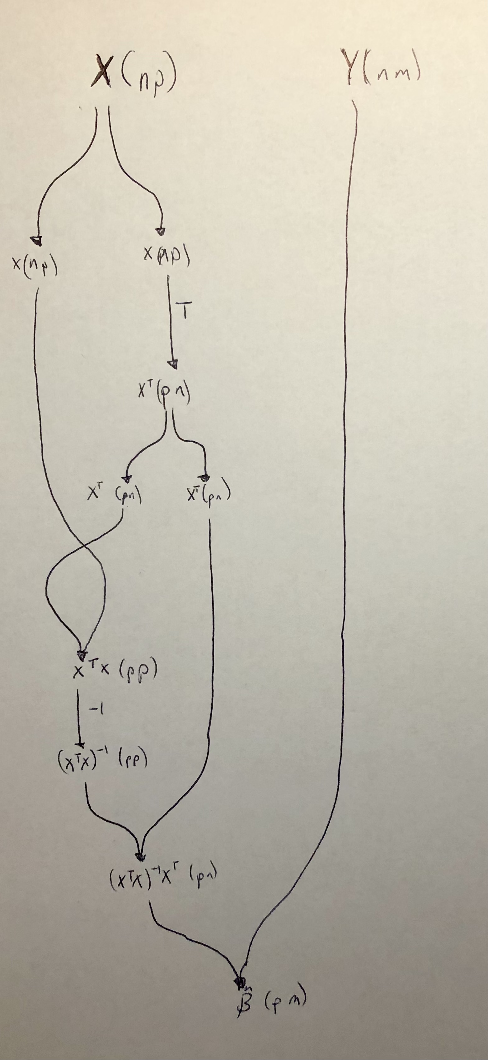
We want to express the following in a categorical way:

\(\hat{\beta} = (X^{\intercal}X)^{-1}X^{\intercal}Y.\)

Here’s a way to do that:

lmFit :: (Cartesian k, Strong k, MatrixPrimitives k
        , KnownNat p, KnownNat n, KnownNat m) =>
    (L n p, L n m) `k` L p m
lmFit = 
  first (copy
        >>> second ( transpose >>> copy)
        >>> ((exr >>> exl) △ exl) △ (exr >>> exl)
        >>> first (compose >>> invert)
        >>> compose)
  >>> compose

This could surely be simplified, but the key (for me) in writing the code above was to first write \(\hat{\beta}\) as a string diagram (see image below). The lmFit code is following along the diagram top to bottom. I’ve included the matrix dimensions in the diagram to make it easier to see what’s happening.

Does it work?

Let’s first try a simple example in Haskell by taking the average for 4 numbers. When the design matrix is a vector of ones, \(\hat{\beta}\) should simplify to the arithmetic mean. Let’s check:

x = matrix 
    [ 1
    , 1
    , 1
    , 1] :: L 4 1

y = matrix
    [ 2
    , 1
    , 0
    , 2] :: L 4 1

test = lmFit (x, y)

Evaluating test in a ghci session results in:

ghci> test
(1.25 :: L 1 1)

Looks good. Let’s try it in R. First we create the lmFit value for the R type. We have to put something for the matrix dimensions. What they are don’t matter; they just need to conform.

r :: (L 4 1, L 4 1) `R` L 1 1
r = lmFit

You can view the result in the test.R script. Testing it out with the same numbers as above:

> catf(list(c(1, 1, 1, 1), c(2, 1, 0, 2)))
     [,1]
[1,] 1.25

Neat. I’ll end by comparing to the built-in lm with multiple regressors:

> X <- matrix(rnorm(100), ncol = 2)
> Y <- rnorm(50)
> catf(list(X, Y))
            [,1]
[1,]  0.04724210
[2,] -0.01312188
> lm(Y ~ -1 + X)

Call:
lm(formula = Y ~ -1 + X)

Coefficients:
      X1        X2  
 0.04724  -0.01312  

Notes

• In principle, I could have started with the least squares objective function and automatically derived the solution (i.e. \(\hat{\beta}\)) using category theory.
• I targeted Haskell and R in my example, but one could compile to Python, Javascript, graphs, and much more.